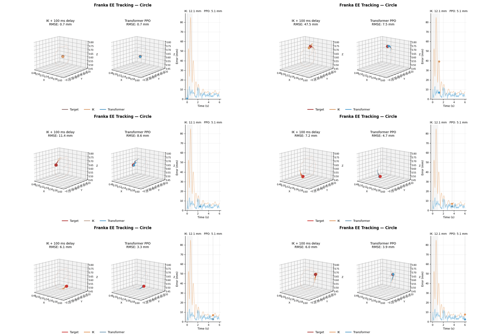
Most robot controllers have a delay. Commands take time to travel through software stacks, buffers, and hardware. For the Franka Panda arm I was working with in MuJoCo, this delay is exactly 100ms — five control steps at 50Hz.
That sounds small. It is not.
The problem
A standard inverse kinematics (IK) controller does something simple: look at where the target is right now, compute the joint angles that would put the end-effector there, send those angles to the robot.
With 100ms of delay, by the time the command reaches the motors, the target has already moved. On a fast random-walk trajectory this causes about 38mm of systematic error — more than double the no-delay case. The robot is always chasing where the target was.
The fix seems obvious: predict where the target will be when the command executes, and command that instead. The hard part is doing this in a way that generalises.
What didn’t work
Delaying only the policy. My first version applied the delay to the RL policy’s corrections only, while IK commanded the robot instantly. The idea was that the policy just needed to fix what IK missed. In practice, IK had a structural advantage the policy could never overcome — it was fighting a delay that IK did not have. No meaningful learning happened.
The fix was simpler than expected: apply the delay to everything. Once IK travels through the same 5-step buffer, it degrades from ~18mm to ~38mm. Now there is a real gap for the policy to close.
Single-trajectory training. A model trained only on the random-walk target reached 20.5mm on that trajectory — but made circle tracking worse than plain IK. The policy had overfit to one distribution. Switching to a mixed training pool (random walk + circle + figure-eight simultaneously) was the single largest improvement in the whole project. It also stabilised the critic dramatically.
The architecture idea
I tried a standard MLP first. It worked, but slowly. After 10 million steps it reached 5.3mm on circle. That is about 55 minutes of training.
The observation space is 95-dimensional. It includes, among other things:
- 5 future target positions spaced 20ms apart (fine lookahead)
- 5 joint setpoints already queued in the delay buffer (command history)
These two sequences have a direct relationship. cmd[i] will execute at exactly the moment fine[i] becomes the current target. The MLP sees both as a flat 95D vector and has to discover this pairing from scratch over millions of steps.
What if we just gave the model that structure directly?
slot[i] = Linear(concat(fine[i], cmd[i])) → 64-dim token
Each token says: “command i will execute when the target is at fine[i].” Feed five of these through a small transformer encoder, and the attention heads can act on that causal link immediately, without having to rediscover which positions correspond to which commands.
At 300k steps, the transformer matched the MLP at 10 million steps on periodic trajectories. 33× better sample efficiency.
The ablation I found most interesting
I ran three ablations, each removing or replacing one component from the canonical architecture (self-attention only, paired tokens, positional embedding):
| Moving Target | Circle | Figure-8 | Verdict | |
|---|---|---|---|---|
| Canonical (self-attn, no xattn) | 24.4mm | 5.7mm | 5.2mm | — baseline |
| A: − positional embedding | 26.8mm | 11.1mm | 10.7mm | PE critical |
| B: + cross-attention | 27.0mm | 5.0mm | 6.5mm | xattn hurts |
| C: unpaired tokens | 26.6mm | 6.8mm | 6.9mm | pairing helps |
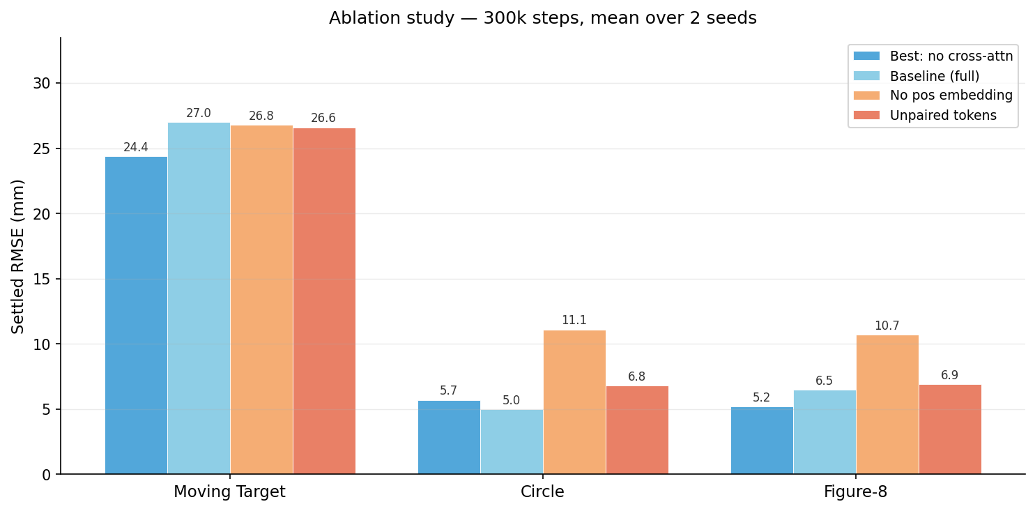
Ablation B surprised me. I had added a cross-attention layer expecting it to help the policy relate its current state to the queued commands. Removing it improved every metric except circle by a fraction.
In hindsight it makes sense. The paired token design already encodes the cmd↔fine relationship directly. Cross-attention was solving a problem that no longer existed. Sometimes the right inductive bias makes a component redundant rather than complementary.
Ablation A was the most instructive failure. Without positional embeddings, slot[0] and slot[4] are indistinguishable to the encoder — the temporal ordering of the delay queue is lost. On periodic trajectories this is catastrophic (+5–6mm on circle and figure-8), because the phase relationship between queued commands is the key signal. Moving target is less affected because random-walk correction doesn’t require slot ordering.
Results at matched compute
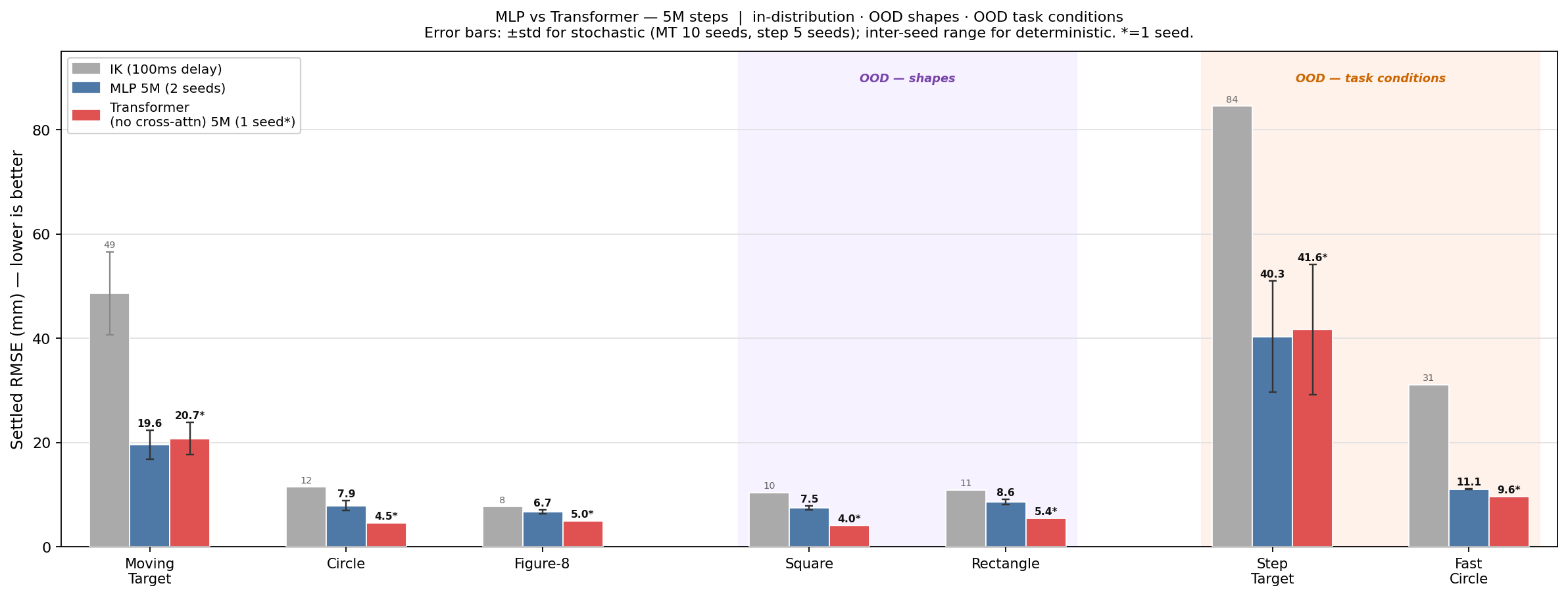
Comparing at 5 million steps, two-seed mean (stochastic trajectories averaged over 10 seeds):
| Circle | Figure-8 | Moving Target | |
|---|---|---|---|
| IK (100ms delay) | 11.5mm | 7.7mm | 48.6 ± 8.0mm |
| MLP 5M | 7.9mm | 6.7mm | 19.6mm |
| Transformer 5M | 4.8mm | 4.8mm | 20.6 ± 3.3mm |
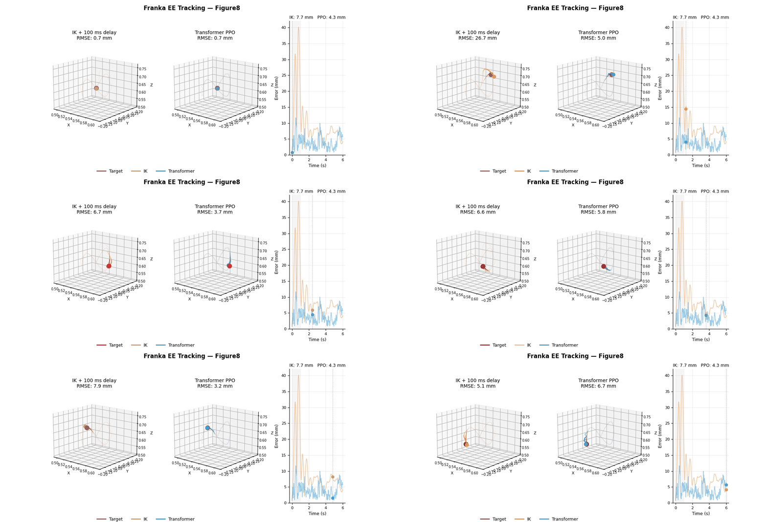
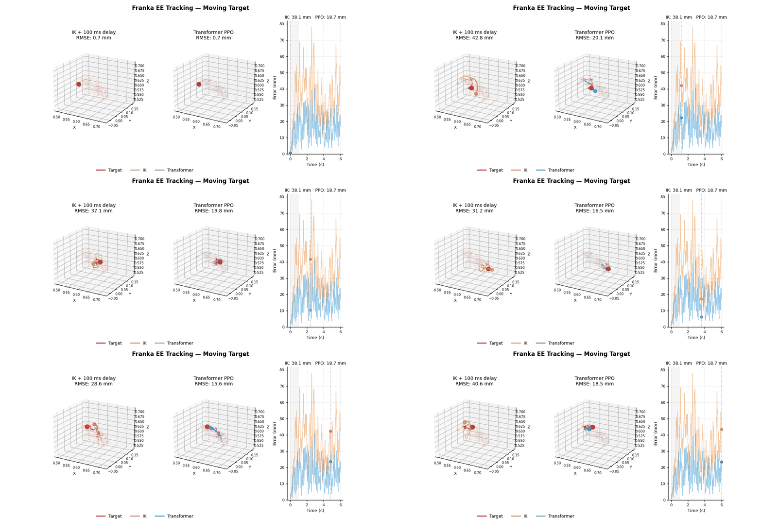
On periodic trajectories the transformer is 39% better on circle and 28% on figure-eight. On random walk, both land around 20mm — essentially tied.
The three training trajectories, transformer policy at 5M steps:
| Circle | Figure-8 | Moving Target |
|---|---|---|
 |  |  |
Out of distribution is where the gap gets larger. On square paths with hard corners (never seen in training), the transformer achieves 4.2mm vs the MLP’s 7.5mm (44% better). The fine lookahead sees the corner 100ms before it arrives, and the transformer uses that information better. The same pattern holds for asymmetric rectangles: 5.1mm vs 8.6mm.
The transformer also produces 38% smoother joint commands (action roughness 0.37 vs 0.60). This came from the architecture, not the reward function — there was no smoothness penalty during training. The paired-slot structure naturally produces less chattering because the policy anticipates rather than reacts.
Does it scale?
I evaluated both architectures at intermediate checkpoints to see how the advantage changes with compute.
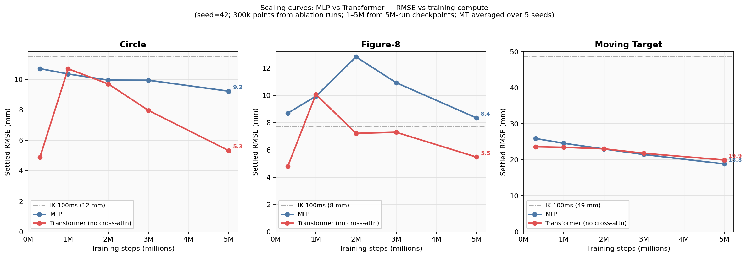
At 1 million steps, both are similar. From 2 million onward the transformer opens a growing gap on periodic trajectories. The MLP keeps improving — it is not stuck — but the transformer is on a better efficiency curve. On random-walk trajectories, they track together throughout.
The story is not “MLP stops working.” It is more that the inductive bias gives the transformer a head start that compounds as it trains.
Honest caveats
The fine lookahead uses oracle future target positions. In a real system you would need a predictor — a Kalman smoother or a learned model. The architecture is set up so you can swap this in without changing anything else.
I have since extended this work to 6-DoF orientation tracking (position + quaternion), where the same paired-slot structure applies with 7D tokens instead of 3D. The orientation task is considerably harder — the IK baseline starts at ~70mm position error and ~30° orientation error under delay — but the same architectural principles carry over cleanly.
What I actually learned
The useful lesson is not “transformers beat MLPs.” It is: if you know something structural about your problem, it is worth encoding that directly rather than hoping the model discovers it.
The delay is fixed and known. The pairing between queued commands and future targets is exact and causal. Wiring that into the token representation — rather than leaving it in a flat 95D vector — gave a 33× sample efficiency gain and cleaner generalisation at the same compute budget.
The delay problem is also more interesting than it first appears. A fixed known delay is actually an advantage: the policy can see exactly how far ahead it needs to look. Variable or unknown delay would be harder. That is a problem I left for later.
Code, pre-trained weights, and full results on GitHub.